CTH v.0.1 — Can’s Third Hardware
I just wanted to hear the voice of the universe.
I heard it.
1. The Algorithmic Lie of the Matrix
It was 2021, the time of COVID. The world had stopped. Back then, I had written a 270+30-page book called Simulacrum. Of course, everything was just theory.
But a book is a book. I wanted to touch it.
I realized I needed random numbers for my TouchDesigner projects: the “random” numbers produced by computers are, in fact, not random at all. They are all the result of a formula. If you start with the same seed value, you get the same numbers — every single time.
This is like trying to generate “random” numbers with a calculator instead of rolling dice. The machine performs a calculation, while the die is a true physical event.
The NSA (National Security Agency) Backdoor
In 2006, the American government released an algorithm: Dual_EC_DRBG (Dual Elliptic Curve Deterministic Random Bit Generator). “This random number generator is secure, use it,” they said. Everyone used it for years — phones, computers, banks.
Then Snowden appeared. It turned out the NSA had put a backdoor into this algorithm. It looked random from the outside, but the NSA could predict all the numbers in advance using a special key.
Think about it: your bank password, your WhatsApp messages, everything — theoretically, it could be read by a single entity. The security of millions of people was left to the mercy of a few.
And this is just one known example. There might not be a backdoor, but “deterministic” (i.e., formula-based) systems are a risk in themselves. An algorithm that seems secure today can be cracked tomorrow.
The answer lies in quantum mechanics.
In the subatomic world, electrons “tunnel” — they exist in multiple places at once, as clouds of probability. Where they will end up is uncalculable — because even the universe itself doesn’t know. This is not a theoretical uncertainty; it is physical reality. The NSA has no backdoor here. It is fundamental, beyond the foresight of even a mythological god.
If you generate a key from a quantum source, no state, no supercomputer can predict it. The universe doesn’t use a formula. It just “happens.”
That is why I started building CTH v.0.1.
2. Tearing the Illusion: PRNG (Pseudo-Random) vs TRNG (True Random) vs QRNG (Quantum)
A computer is essentially a boring thing. If you ask the same question, you get the same answer — every time, for years, forever. It cannot generate randomness. It can only imitate it.
PRNG: Pseudo-Randomness
PRNG — pseudo-randomness. A formula, a seed value. You call rand(); the computer actually does this: seed = (seed * 1103515245 + 12345) % 2^32. The same sequence every time. The same start, the same finish.
A rigged die. It has a mechanism inside, repeating the same pattern every time you roll it. If you watch long enough, you can predict it.
TRNG: Hardware Randomness
What if you take readings from real physical events? This is TRNG — keyboard timing, fan noise, atmospheric noise, thermal vibration in a resistor.
A good start. But it’s slow, some are susceptible to manipulation, and deterministic components can creep in.
QRNG: Quantum Randomness
The purest form: QRNG. Directly measuring the universe’s own indeterminacy.
No one knows where an electron will be — there is a probability distribution, but no result. “Indeterminacy” is not an abstract concept; it is within the silicon, instantaneous, and non-repeatable physical events.
CTH v.0.1 measures the quantum tunneling noise of 2.4V zener diodes. The sound of the universe’s own “decision-making” process.
Summary Table
| Type | Source | Predictable? | Reliable? |
|---|---|---|---|
| PRNG | Mathematical formula | Yes (with key) | No |
| TRNG | Physical noise | Difficult but possible | Moderate |
| QRNG | Quantum indeterminacy | Impossible | Yes |
All modern cryptography — your encrypted messages, bank transactions, VPNs — is built on these RNGs. And most still use PRNGs. Which means we are living inside a giant illusion.
Cryptography = The Foundation of Civilization
Encryption isn’t just about your WhatsApp messages. Banks, elections, military orders, nuclear codes, health records — all stand on this same foundation.
Remember what happened when banks collapsed in 2008. Now think: if cryptography collapses, accounts disappear, elections change, orders are forged. A great, silent collapse. No one notices because everything looks like numbers.
RNG is the cornerstone of this foundation. No matter how magnificent the building is, if it’s built on a rotten foundation, it will eventually crumble.
The Human Brain Fails, Too
“Okay, but I can say a random number.”
No, you can’t.
The brain searches for patterns. It hates randomness. If I asked you for a sequence of numbers: 3, 7, 12, 4… You never repeat the same one consecutively, you cluster around small numbers, you create rhythm — like 4, 8, 12. You avoid “ugly” numbers like 87 or 93. Statisticians have tested this many times. It is predictable.
We are PRNGs too. We just work with more complex formulas.
3. Zener Mechanics: Two Breakdowns, Two Different Universes
Why 2.4V? Why not “avalanche”? This is the heart of the project.
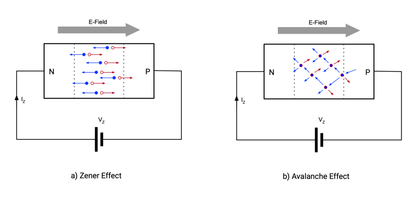
Zener Breakdown vs Avalanche Breakdown
When diodes are reverse-biased (voltage applied in the opposite direction), a “breakdown” occurs at a certain point. There are two types:
| Feature | Zener Breakdown | Avalanche Breakdown |
|---|---|---|
| Voltage | Low (< 5.1V) | High (> 5.1V) |
| Mechanism | Quantum Tunneling | Avalanche Collision |
| Physics | Electron tunnels through | Chain of electron collisions |
| Temperature | Voltage DECREASES as it rises | Voltage INCREASES as it rises |
| Noise | Pure quantum indeterminacy | Thermal + classical chaos |
Quantum Tunneling: Finite Square Well
To understand what happens in a zener diode, let’s start with a simple model: the finite square well.
Think: An electron is trapped between two walls. In classical physics (Newtonian mechanics), if the electron’s energy is less than the wall height, it is impossible for it to get out. It hits the wall and bounces back. It stays inside forever.
But in quantum mechanics, the situation is different.
Schrödinger Equation
The equation defining the electron’s behavior:
Where:
- = Planck’s constant /
- = electron mass
- = wave function
- = potential (barrier)
- = electron energy
Classically Forbidden, Quantally Permitted
In a finite square well, the potential is defined as:
Classical physics: If , the electron can never cross the barrier.
Quantum: The wave function is not zero in the barrier region. It decreases exponentially but never hits zero:
Meaning, on the other side of the barrier, there is a probability that the electron exists!
Tunneling Probability
If the barrier width is , the transmission coefficient for the electron is:
This is a random process. For a single electron, whether it crosses or not is uncertain. Two electrons with the same energy, at the same barrier — one crosses, one bounces back. The universe decides this by “rolling the dice.”
As you see in the video, the particle crosses the barrier — impossible in classical physics. But possible in quantum. And when it crosses is indeterministic.
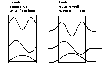
In the animation above, you see the finite square well. Note: The wave oscillates inside the well (the electron is here), but the wave is not zero to the left or right of the walls — it decreases exponentially. That “wave outside the well” is the probability of tunneling.
Zener Diode: Tunneling in Real Life
What is a Zener Diode?
A Zener diode is a special semiconductor that “breaks down” at a specific voltage when connected in reverse bias (cathode positive, anode negative). Normal diodes break down and burn in reverse voltage, but a zener does this in a controlled way and survives.
Basic use: Voltage regulation. A 2.4V zener clips voltage above 2.4V at the cathode and keeps it constant. But for us, another feature is important: its reverse noise.
Production and Depletion Region
A Zener diode consists of a junction between p-type and n-type semiconductors (PN junction). In this junction, carriers (electrons and holes) diffuse and neutralize each other. The result: the depletion region — a carrier-less region that acts like an insulator.
The width of the depletion region () determines the zener voltage:
- Thicker region → Higher voltage required for breakdown
- Thinner region → Breaks down at lower voltage
Formulaically:
Where (acceptor) and (donor) are doping concentrations. The higher the doping, the thinner the depletion, and the lower the zener voltage.
Why is 2.4V the Physical Limit?
Lower voltage requires higher doping. But there is a physical limit to doping:
- Solid solubility limit: You can’t replace so many atoms with dopant atoms in silicon — the crystal structure degrades.
- Band gap limit: Silicon’s band gap is ~1.12V. The Zener voltage cannot drop below this (physically impossible).
- Tunneling distance: If the voltage is too low, the depletion region becomes extremely thin. So thin that tunneling becomes guaranteed, and the diode behaves like a “short circuit.”
2.4V is near these physical limits — still controllable in production, but anything lower is either impossible or useless. There are 2.0V or 1.8V zeners on the market, but their tolerances are very loose (like ±20%) and stability is poor.
2.4V is at the limit of the “lowest stable voltage achievable.” And I am using this limit — because it’s the region where quantum tunneling is purely dominant.
Avalanche Breakdown: The Avalanche Effect
At high voltages (5.1V and above), electrons accelerate and collide with atoms. Each collision frees new electrons. A chain reaction — an avalanche.
Why it’s a problem:
- Actually, avalanche has quantum mechanics too — the electron ejection starts via a quantum effect.
- But this is an “ugly” quantum. It’s a chain reaction, the chaotic motion of millions of electrons.
- The thermal component dominates the noise — a “noisy” signal at the mV/√Hz level.
- Most “quantum” RNGs on the market use this method — amplify by 10x and go.
Temperature Response: The Critical Difference
Here is the litmus test: when the temperature changes, the two breakdown types react in opposite ways.
Zener (Quantum):
- If temperature rises → Breakdown voltage DECREASES
- Negative temperature coefficient
- Why? Tunneling probability increases with temperature.
Avalanche (Classical):
- If temperature rises → Breakdown voltage INCREASES
- Positive temperature coefficient
- Why? Atomic vibrations increase, collisions become more difficult.
This difference is used to test which mechanism is at work. I performed a temperature test on my 2.4V zeners — I verified the negative coefficient. Because it shows variable reactions depending on ambient temperature, I had to include an IC that performs both calibration and temperature measurement.
Why 2.4V?
The nominal threshold where zener breakdown starts is around ~2.7V. But it’s a spectrum:
- 2.4V: Pure zener breakdown region — entirely quantum tunneling.
- 3.3V: Still zener dominated, but a small avalanche component begins.
- 5.1V and above: Avalanche completely dominates — the world of classical physics.
Why is Avalanche Impossible Below 2.7V?
For avalanche (the chain effect) to occur, there needs to be a distance for electrons to accelerate enough. An electron must gain momentum to collide with atoms and knock other electrons loose — that is, it needs a certain length to accelerate.
In zeners below 2.7V, the depletion region is so thin (~nanometers) that the electron passes through before it can accelerate in this narrow corridor. There isn’t enough “runaway” distance. Therefore, the only mechanism is quantum tunneling.
At 2.4V, the depletion thickness is at the edge of the theoretical limit. If it were any thinner, the diode wouldn’t operate stably; if it were any thicker, it would already be a higher voltage.
Actually, 2.4V isn’t a “sweet spot” — it’s the most impossible place. The lowest zeners sold on the market are 2.4V. Even if there are lower ones, they are at the theoretical limit (max ~2.0V), stability is zero, and tolerances are around ±20%. Manufacturers don’t even want to go to this limit.
I did something crazy and stuck exactly to this limit. Because at the limit of physics, quantum tunneling is the purest.
Noise Dynamics: Whisper vs Noise
Here is the critical difference: the noise character of the two mechanisms is completely different.
Avalanche Breakdown: High-energy ions knock electrons loose, initiating a chain reaction. This is a very noisy process:
- Noise level: mV/√Hz (millivolts per root-Hertz)
- Meaning quite high-amplitude noise
- No need for delicate amplification
- This is why “TRNG” devices on the market use this — connect, amplify, send.
Zener Breakdown (2.4V): Pure quantum tunneling. Electrons pass one by one, silently:
- Noise level: nV/√Hz (nanovolts per root-Hertz)
- This is thousands of times quieter than avalanche.
- A true “whisper.”
- But this whisper is the universe’s own voice.
Numerically: 1 mV = 1,000,000 nV. Avalanche noise is ~1000x higher in amplitude than zener noise.
Devices on the market use 12V, 15V, 24V (the full avalanche region). Then they amplify this signal 10x, and move on. This is sufficient. The signal is already strong.
I can only hear 2v4 zener noise with 250-300x gain, meaning I amplify it 250-300 times.
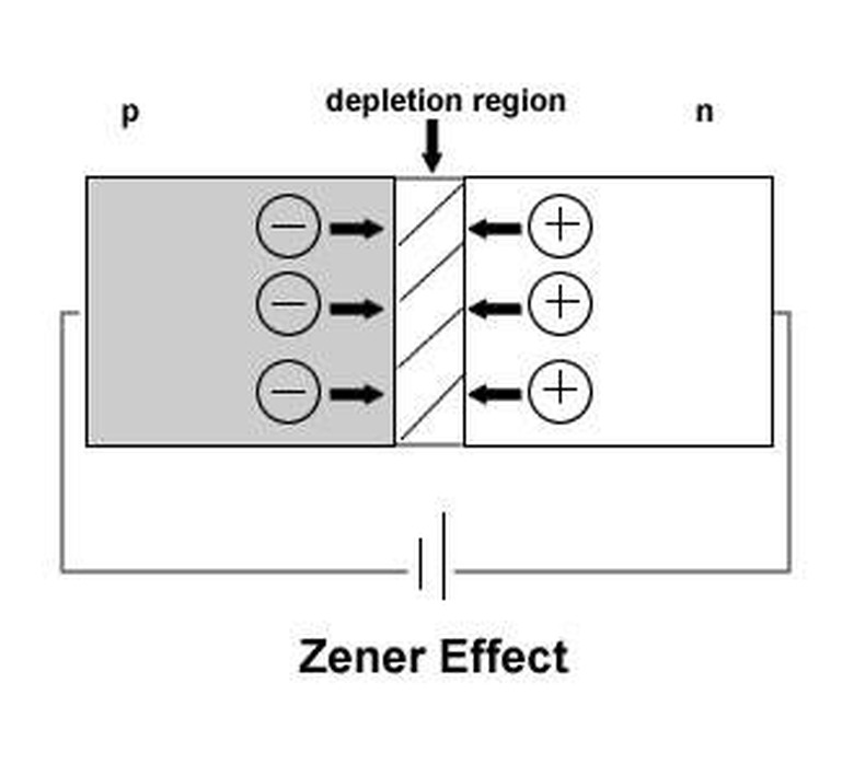
As you see in the graph above, the zener region creates a sharp “knee.” In this region, small voltage changes produce large current changes — and these current fluctuations are a direct measurement of quantum indeterminacy.
4. Black Magic: Analog Electronics
Theory is over. Now for the real work: hearing the quantum whisper at the nV/√Hz level.
Digital vs Analog: Two Different Universes
In the electronics world, analog engineers are called “black magicians.” And analog design is called “black magic.” Why?
The digital world — 0 and 1. Precise, clear, predictable. You write code, it works. If there’s an error, the debugger finds it. Everything is deterministic. Voltage > 3v = 1, Voltage < 1.5v = 0.
The analog world — exactly the opposite. Everything is fragile and unpredictable.
With a capacitor and a resistor, you perform calculus operations like derivatives and integrals in the analog world. The operation that makes digital computers struggle with thousands of calculation steps, an analog circuit performs instantly, in continuous time. But…
When you open the window in the room, the calculation changes. Because:
- Every copper trace is an antenna — it picks up radio frequencies.
- Your finger is a capacitor (at the pF level) — the signal changes where you touch.
- Humidity, temperature, pressure — shift resistance values.
- Mains power (50 Hz) — leaks into everything.
- The neighbor’s drill — produces instantaneous voltage spikes.
- Your own phone — WiFi/Bluetooth interference.
There is no isolation in an analog circuit. Everything talks to everything else. The output of an op-amp is affected by ripples in the power line. A filter capacitor changes with the heat of your hand.
In digital, once you say “it works,” you’re done. In analog, when you say “it works,” you wait until you close the door to the room.
Johnson Thermal Noise: Standing Still is Forbidden in the Universe
One of the most fundamental magics of the analog world: Johnson-Nyquist noise.
Even a resistor that is sitting there doing nothing, with no voltage applied, lying on the table — due to the thermal motion of the electrons inside — produces continuous noise. If you connect it to an oscilloscope, expecting a horizontal line, you see a small “fluctuation.” This is the universe’s own silent whisper.
Its formula:
Where:
- = Boltzmann constant (the universe’s temperature constant)
- = temperature (Kelvin)
- = resistance (Ohm)
- = bandwidth
Meaning: Standing still is forbidden in the universe. Every electron is constantly vibrating. Even if every material looks motionless, it dances at the microscopic level.
Example calculations (room temperature ~300K, 10 kHz bandwidth):
- 1kΩ resistor: ~400 nV (nanovolts) noise
- 10Ω resistor: ~13 nV noise!
- A plucked human hair (when dry, ~10¹² Ω insulator): ~13 mV noise!
Yes, a plucked hair — which seems disconnected from the circuit because it’s an insulator — actually produces thermal noise. Because there is no such thing as a truly “insulating” material in the universe, only “very high resistance.”
In my project, this noise is both an enemy and a friend:
- Enemy: The zener’s nV/√Hz noise can be lost within this thermal noise.
- Friend: If the zener noise is higher than this thermal floor, the real signal can be distinguished.
That’s why low temperature, low resistance, narrow bandwidth — everything is critical.
Why Two Zeners? — “I Couldn’t Know Without Testing”
At first, I thought about a single zener. But there was a problem: I didn’t have an oscilloscope.
I only had a cheap logic analyzer and an STM32 SWD debugger. These tools can see digital signals, but they can’t measure analog noise. How was I going to be sure that what I heard was truly random?
This is where math stepped in. I knew information theory: The XOR of two independent random sources is also random. Its entropy even increases:
Meaning: If a single zener produces truly random numbers, the XOR of two zeners must also be random. And if there is a “pattern” (bias) in a single zener, the second zener “mixes” this pattern.
That’s why I designed two channels. Each zener is independent:
- Physically separate components.
- Separate amplification chains.
- They arrive at the same ADC (Analog-to-Digital Converter) and are XORed in software.
But there is another reason for this: Security. An electromagnetic attack (EM pulse) can be directed at a single zener. But interfering with two independent channels at the same time is much harder. This provides “fault tolerance” (if one channel fails, the other continues) and protection against “side-channel attacks.”
The Realities of Parts On-Hand vs Market Parts
In the analog war, you need very good tools. But what did I have on hand?
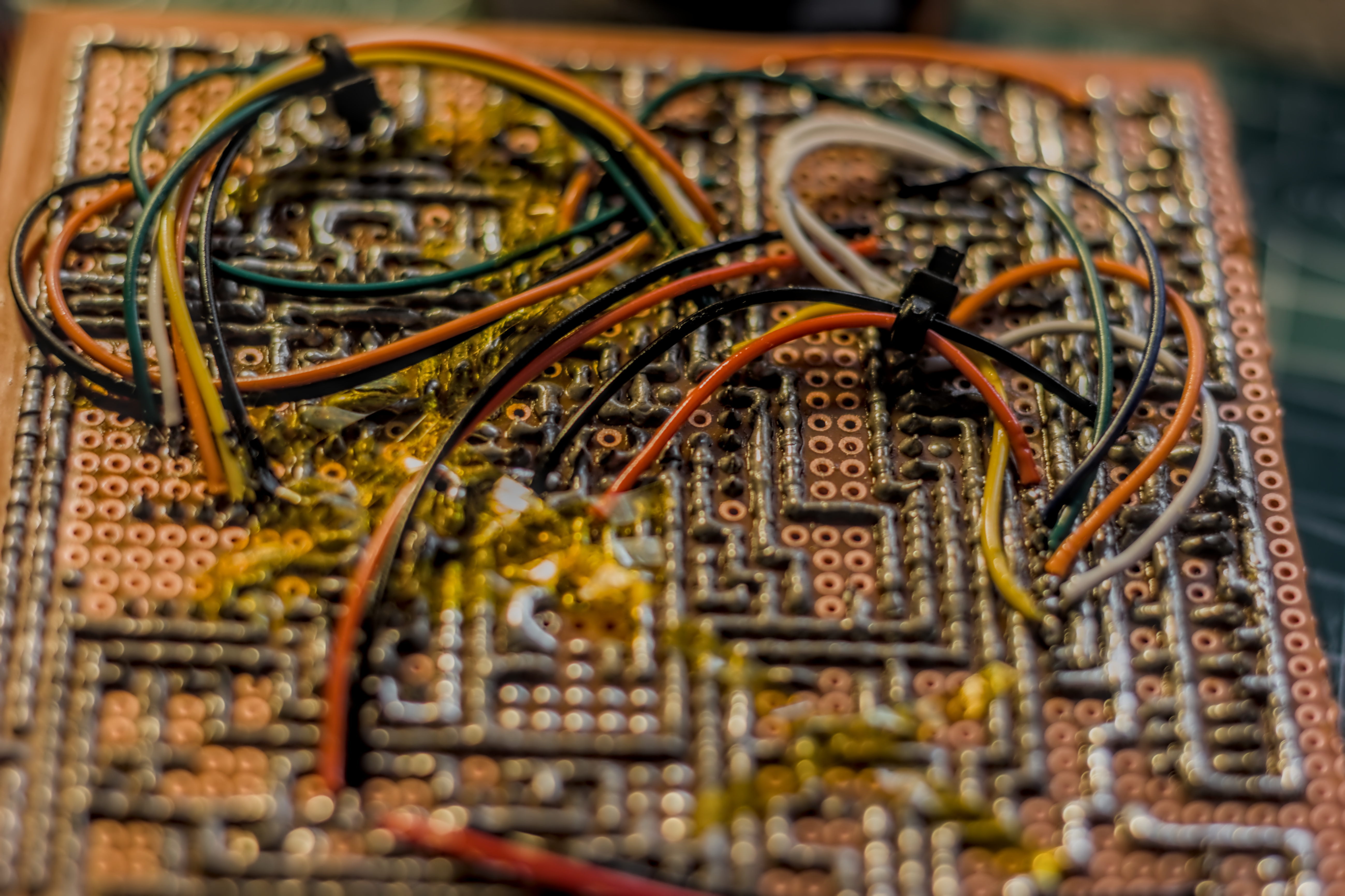
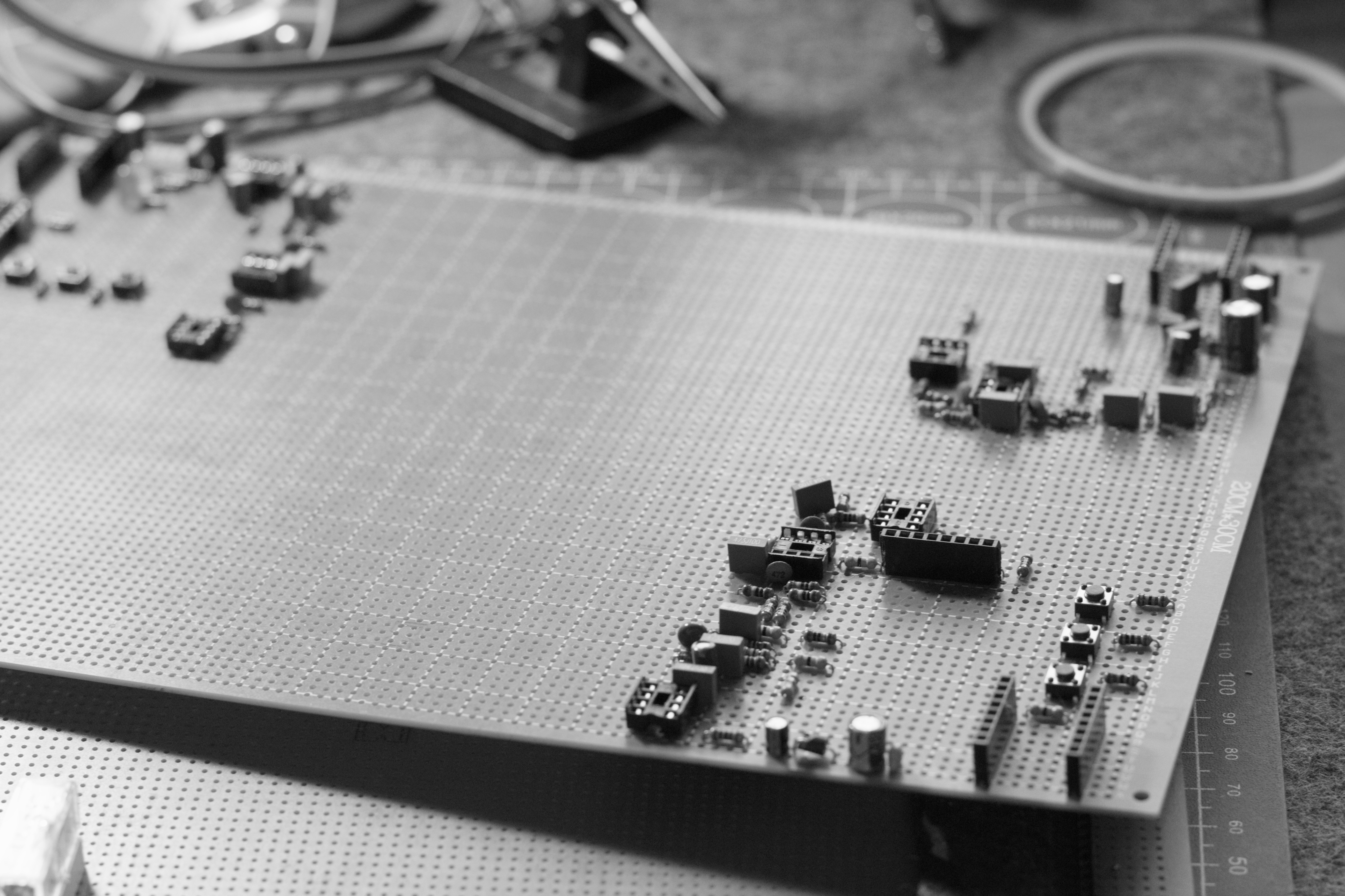
Pertinax: Chinese FR2 single-sided, straight out of 1980s Soviet gear. Instead of quality FR4, old-school fireproof board. No impedance control, poor signal integrity. But cheap and accessible.
Op-Amp: The lowest-noise IC I had was ~8.7 nV/√Hz. Theoretically “low-noise,” but in reality… Comparison: “Audio grade” op-amps on the market do 3-4 nV/√Hz. But those are expensive and hard to find.
Zener breakdown noise varies between 20-100 nV/√Hz. The op-amp’s 8.7 nV noise can be lost within the zener signal. That’s why:
- Choosing a low-noise op-amp is a must.
- Narrowing the bandwidth (narrow band = less noise).
- Keeping the temperature low (cold = quiet).
The Rail-to-Rail Nightmare: Op-amps usually want symmetrical supply (+V and -V). There are voltage pump ICs to generate negative voltage, but they are… incredibly noisy. Worse than Johnson noise on their own.
Solution: Use rail-to-rail op-amps. These work with a single positive supply (between 0V and 5V). But the disadvantage of rail-to-rail: usually higher noise. 8.7 nV is considered “good” in the rail-to-rail world.
Zener Variety: I bought products from 3 different manufacturers all labeled “2.4V zener.” Each has a different noise character! Some are 20 nV, some 80 nV. Maybe they were produced in the same factory, maybe not. This is the “black magic” of the analog world: even two parts with the same label aren’t the same.
So in this war:
- The pertinax is low quality.
- The op-amp is noisy (but the best I had).
- The zeners are inconsistent.
- Symmetrical supply is impossible (due to noise).
- You can’t choose every resistor; even a single resistor can produce 100 nV of noise on its own.
The Curse of DC
When zeners work, they produce a DC offset around ~1.25V. But I am interested in the AC noise — the microscopic fluctuations around this DC.
The first problem: Getting rid of this DC. If I amplify it directly, the op-amps go into saturation. Solution: a passive RC filter: cutoff ~10-15 Hz. Both DC (~0 Hz) is completely blocked, and most of the zener noise spectrum is preserved.
At this point, everything is connected: HPF (High Pass Filter) is needed to block DC, a resistor is needed for the HPF, the resistor produces Johnson noise, which is why the resistance value is critical…
nV to mV: The Gain Nightmare
2.4V zeners produce nV/√Hz noise. The STM32’s ADC (Analog-to-Digital Converter) expects a signal at the mV level. The chasm in between: 250-300x gain is necessary.
300x in a single stage? Impossible. Chaos of stability occurs, oscillations begin. Solution: multi-stage amplification: ~50x first stage, intermediate filters (for phase compensation), then ~5-6x second stage. Total 250-300x.
Impedance matching between each stage is critical: . If they don’t match, the signal weakens, and the frequency response deteriorates. Op-amp buffer circuits provide this isolation.
Drawing the Bandpass by Hand
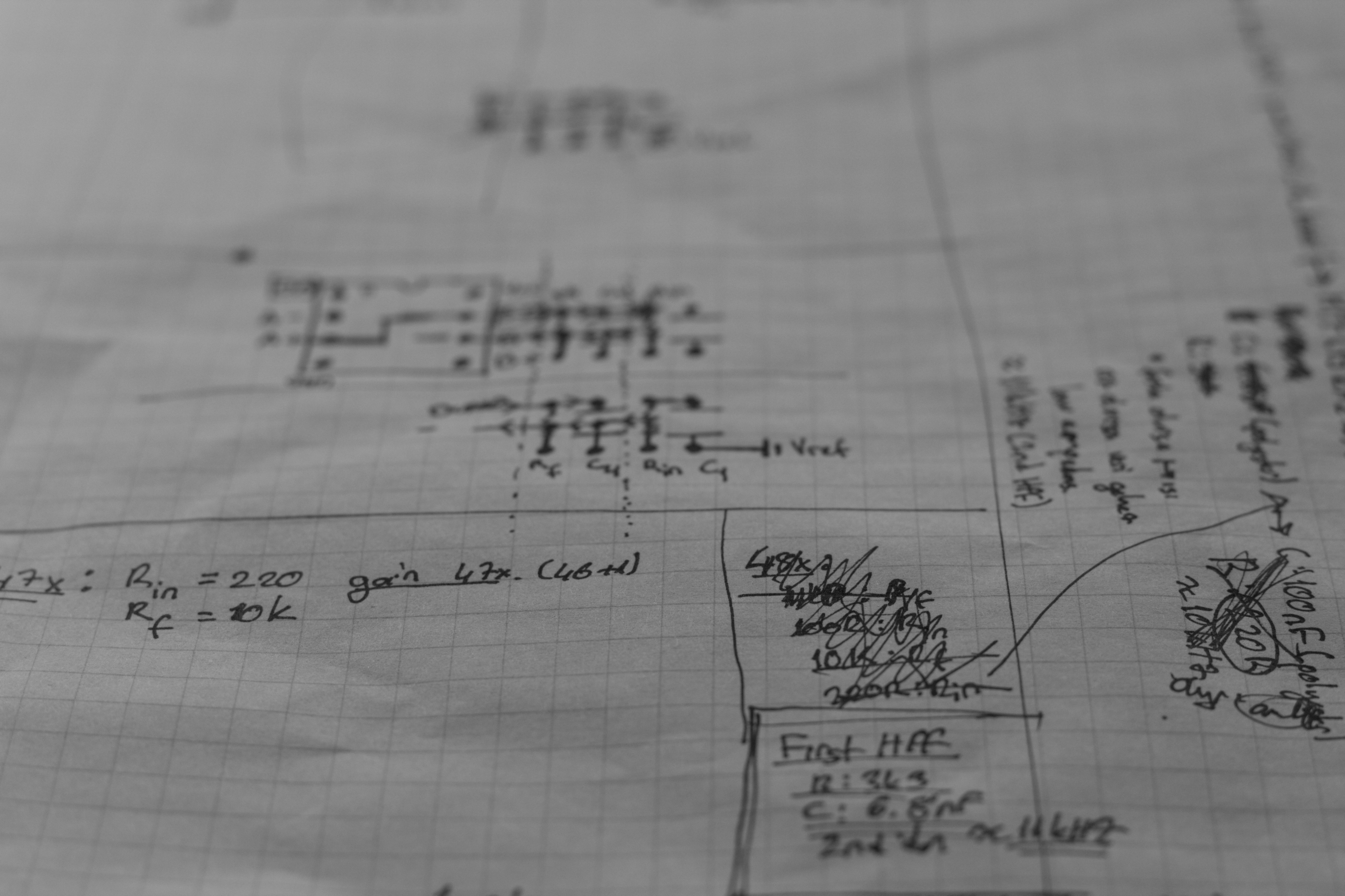
I designed active filters to shape the noise spectrum. The HPF (High Pass Filter, ~10-15 Hz) blocks DC and mains ripple. The LPF (Low Pass Filter, ~10-20 kHz) cuts off RF interference and prevents sampling errors. Together, they behave like a 10 Hz - 20 kHz bandpass.
I made dozens of attempts while calculating and soldering these filters. 3-4 circuits went into the trash. Some oscillated, some ruined the frequency response, some increased the noise. Tolerances of passive components (±5%, ±10%) really distance the theory from reality. Finally, I achieved a stable chain.
STM32: Transition to the Digital World
The final stage: STM32F103 (Blue Pill) 12-bit ADC (Analog-to-Digital Converter). 3.3V reference, ~0.8 mV LSB (Least Significant Bit), 48-96 kHz sampling. The amplified signal (~mV level) can be read directly. 48 kHz sampling = captures frequencies up to 24 kHz, covering 95% of the zener noise spectrum.
And this entire chain — without an oscilloscope, designed only with a logic analyzer and math.
The Hell of Min-Maxing: Resistors and Fatal Choices
In the analog world, every choice has a price. This project turned into an optimization hell of those prices.
High resistance → High Johnson noise (remember: ). A 100kΩ resistor alone produces 100+ nV of noise. The zener signal gets lost in this sea of noise.
Low resistance → Loading effect. When you load a very low impedance onto a zener diode, the source impedance affects it. The zener’s “breathing” is ruined, and the noise is destroyed.
This is the dilemma: Very high resistance = interference noise. Very low resistance = source dies. To find the optimum point…
3 Prototypes, 3 Trash Bins
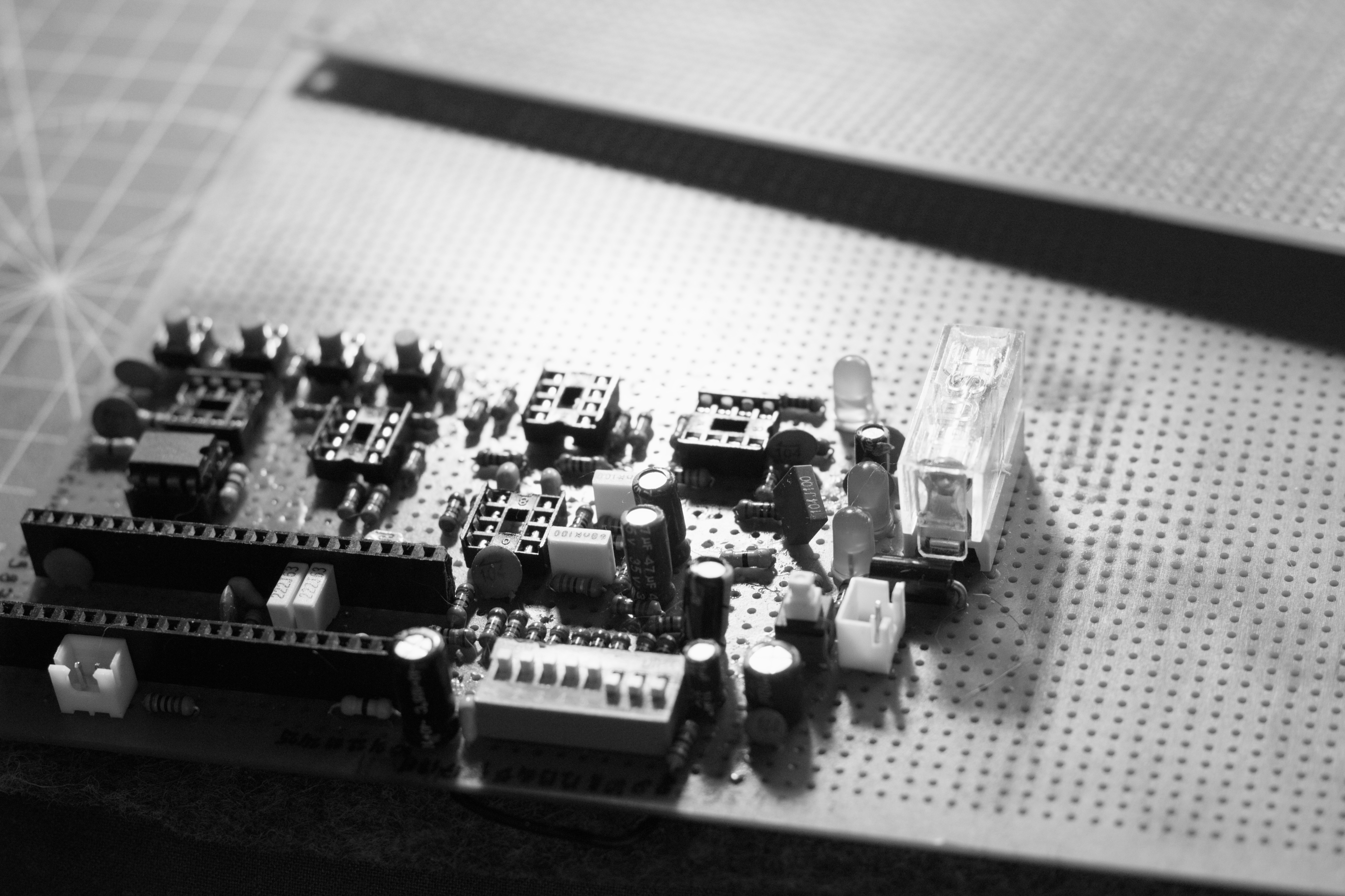
I built and disassembled 2-3 different prototypes. LEDs were flashing, the STM32 code was running, data was flowing. But when I ran the entropy test: 5-6 bits.
Theoretically, you cannot see higher than 8 bits/byte of entropy in this universe. This is the theoretical limit of randomness (2⁸ = 256 states). My goal was 7.9+ bits.
But 5-6 bits? This means a “deterministically appearing random” signal. Maybe power supply ripple, maybe RF interference, maybe op-amp oscillation. The real quantum noise was lost beneath these impurities.
Every time a prototype went into the trash, I found the reason:
- In one, the resistor values were wrong, Johnson noise became dominant.
- In one, the filter cutoff was too narrow, cutting off half the zener spectrum.
- In one, PCB isolation was bad, the mains leaked into everything.
Gain Control: From Trimpot to Mux
Constant gain adjustment was required. Because the word “tomorrow” is dangerous in the analog world. Humidity changes, temperature changes, resistance values drift. A circuit that worked perfectly yesterday might go haywire today.
Trimpot? Carbon composition. Produces 100+ nV noise on its own. Impossible.
Digital pot? Switching noise. The switches inside produce sudden spikes at every transition.
I thought about it for weeks. Then the solution came: Analog Mux + 16-resistor ladder.
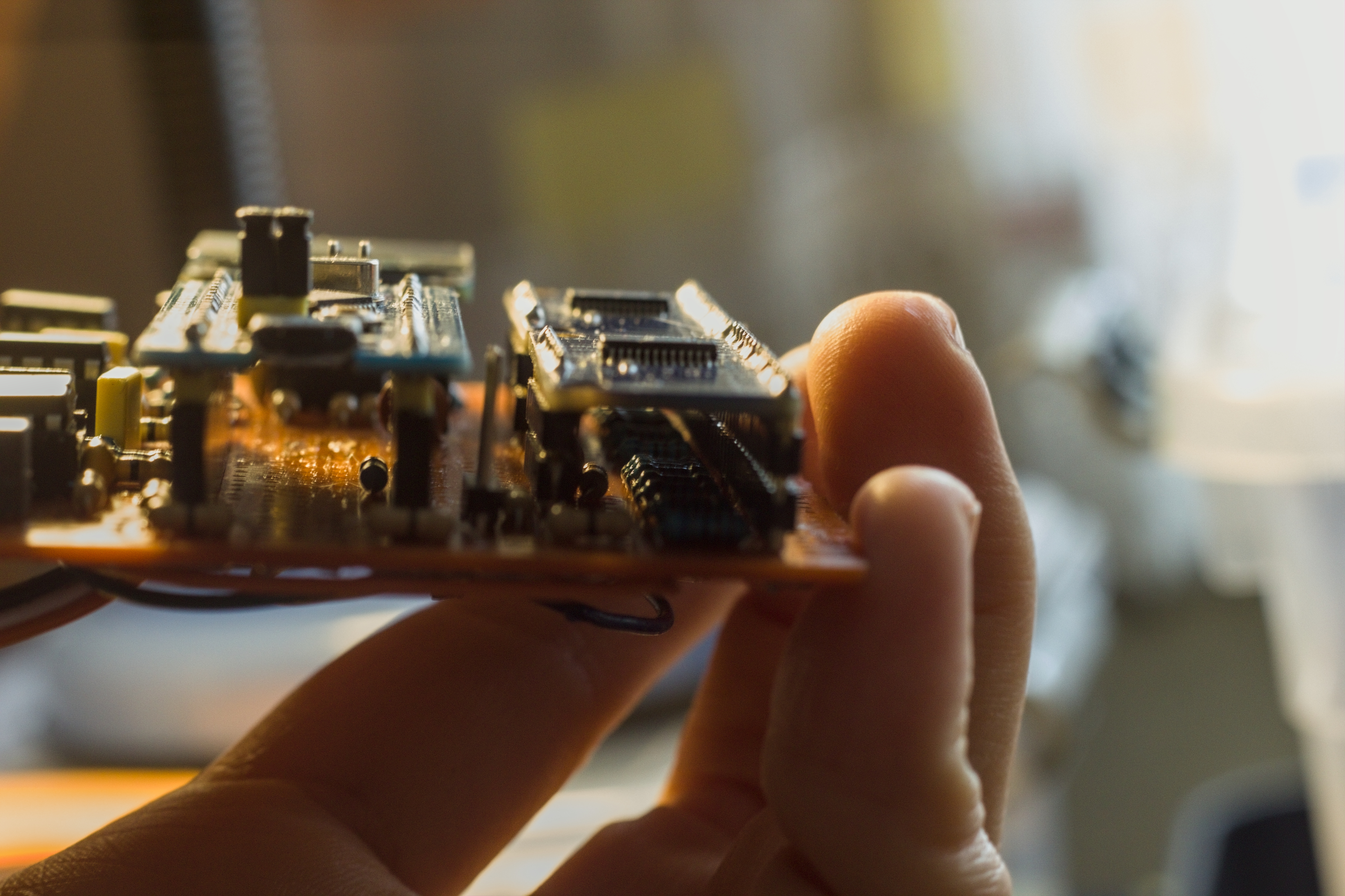
74HC4067 multiplexer + 16 pieces of 1% precision metal film resistors. The mux selects 16 different resistor combinations with 4-bit digital control. Each resistor path has Johnson noise, but… this noise can be calculated and characterized. And it is stable.
No switching noise because the mux only makes the selection, not during the transition. No carbon noise because I’m using metal film resistors (thin film).
Current Control: The Zener’s Breath
The operating point of Zener diodes is critical. Too low current = can’t enter the breakdown region, produces no quantum noise. Too high current = heats up, thermal noise increases, stability is ruined.
But current control was a total headache.
In early circuits, I wanted to drive the zeners with classic voltage control. Zeners have dynamic internal resistance dependent on voltage — resistance drops as voltage rises, increases as it decreases. But this is entirely random, dependent on production tolerance.
The result? In my first circuit, the zener that had less resistance at that moment always STOLE the current the other one deserved!
Yes, two zeners side-by-side, at the same voltage, but one is “greedier” than the other. I forced them to share with series resistors. It seemed to work, but… the entropy test was still pathetic. 5-6 bits, sometimes lower.
I thought about it for 1-2 weeks. What was the problem? In those days, I told myself, “Switch to Avalanche, this is impossible, just quit!” But I didn’t give up.
One night, at 3 AM, it hit me: The problem was in the op-amp’s output impedance!
Theoretically, the op-amp output should be “zero impedance.” Look at it from the zeners’ perspective: The “thing” providing power is lower resistance than you! When that happens, that tiny quantum noise remains on the zener, is seen by the op-amp as an “error,” and is wiped out! The op-amp was trying to “correct” the zener’s noise.
The solution? Show the op-amp’s output as “infinite impedance” to the zeners. Meaning:
If (constant current source), then !
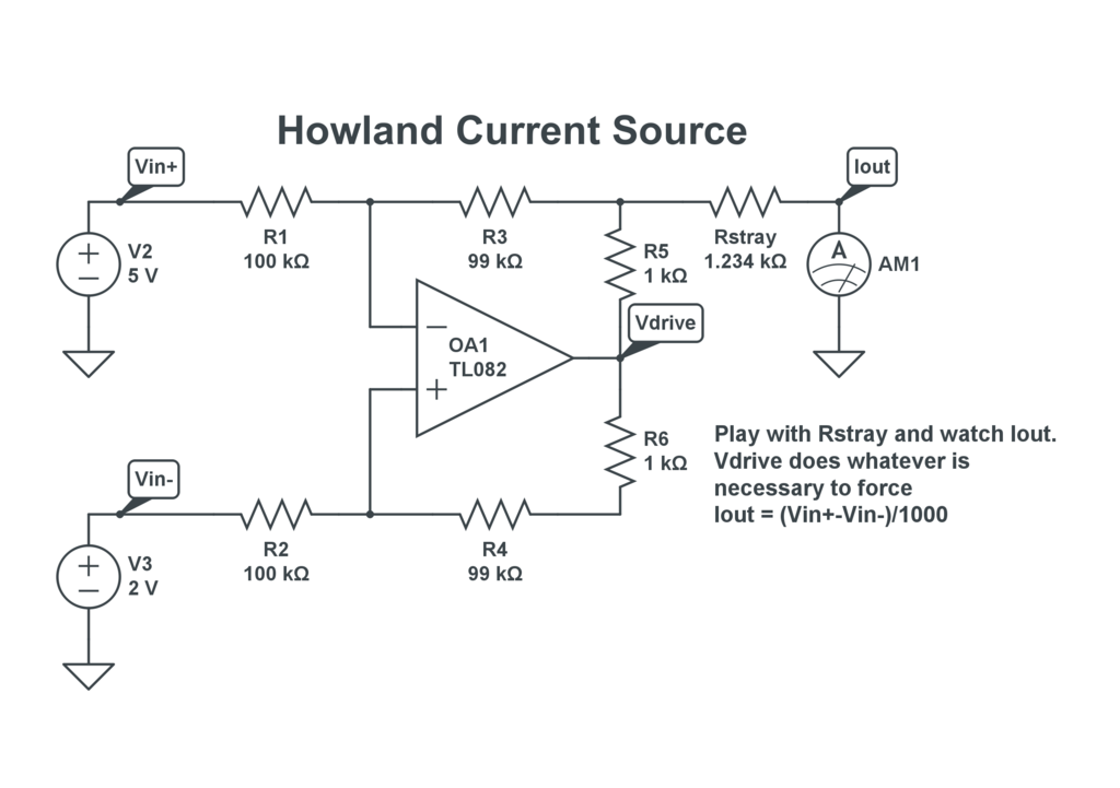
I researched, researched… Symmetrical VCCS (Voltage Controlled Current Source)! Yes, theoretically this worked. From the zeners’ perspective, the op-amp is now “floating,” with infinite impedance.
But… in this topology, the zeners are not connected to ground (chassis), they are “floating.” This causes new problems. Then I found the Howland Current Source topology. It sounded perfect.
But… even if the resistors used in Howland are 1% precision, if they differ slightly from each other, the impedance crashes to the ground! Theoretical formulas are perfect on paper, but real resistors…
This is also the curse of the analog world: Math is perfect, materials are a disappointment.
Finally, after days of trial and error and calculations, I achieved a modified Howland current source topology that wasn’t perfect but was good enough.
I won’t talk about the “trick” I used here 😉🤫 — it’s a trade secret, right? xD
Dynamic Current Control: Software-Tuning the Zener’s Breath
Of course, this topology is not enough; you need to control the current dynamically!
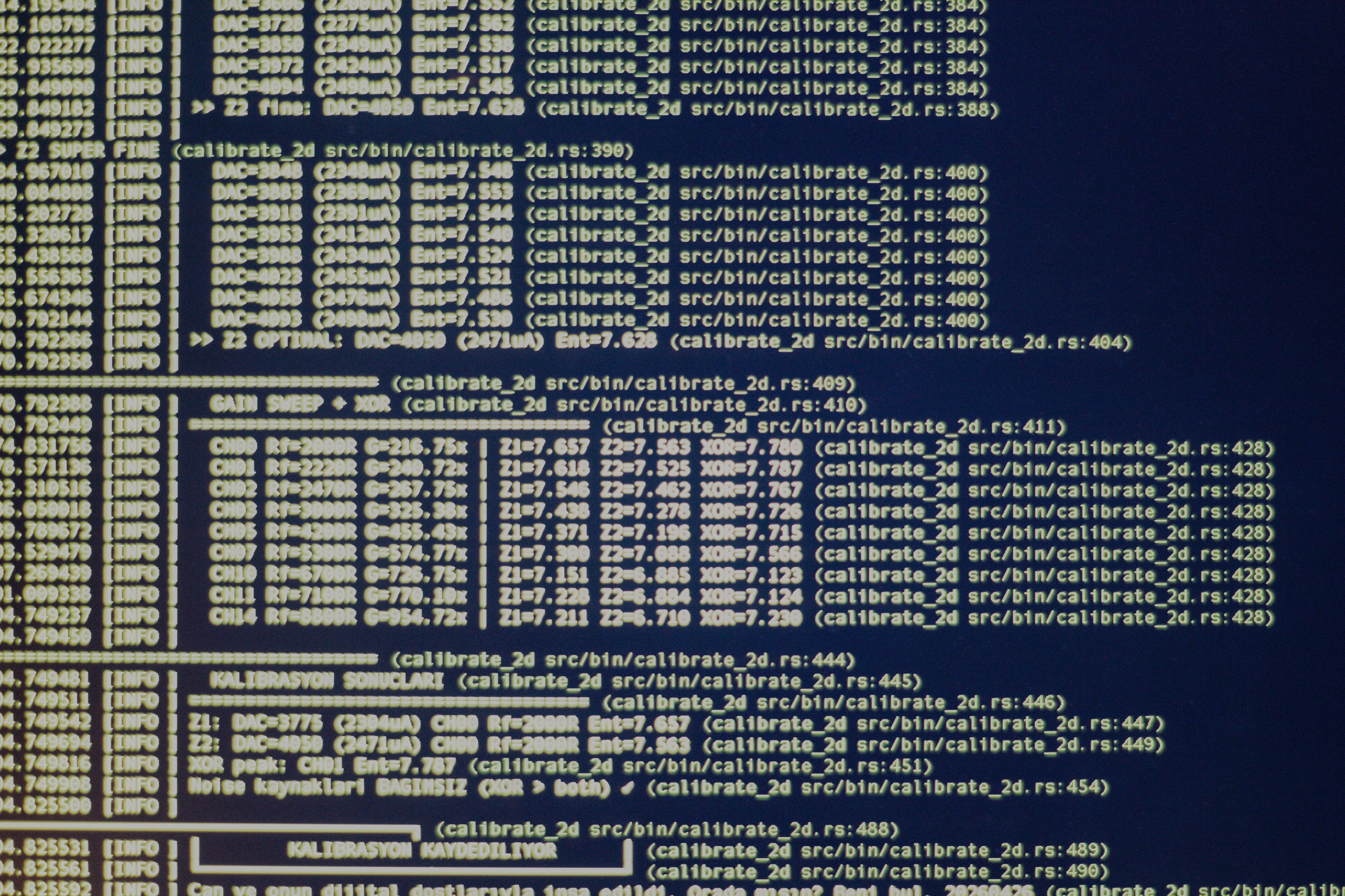
To make this stable, you need a separate DAC (Digital-to-Analog Converter) chip. Classic PWM + RC filtered DAC has ripple issues. I used a 2-channel 12-bit DAC IC and controlled the current to max 2.5mA per zener. 12-bit resolution means 4096 steps (2¹²) — meaning per step:
I could adjust the zener current with 0.6 microamp precision per step! This allowed me to control the operating point of a single zener with microscopic meticulousness.
Together with analog mux gain control, calibration was now 2D; I could dynamically adjust both current and gain in software. This two-dimensional control space allowed me to optimize entropy performance at different operating points.
Filter Design: The Only Way to Listen to the Universe
The most critical stage for listening to this noise is the filter — HPF (high pass) and LPF (low pass). This design determines the fate of everything.
Because whether you realize it or not, we live in an extremely noisy world. The sources of electromagnetic interference in the room where you are right now:
- 50 Hz mains noise — constant frequency signal emitted from every socket on the wall, lighting, motors.
- Switched-mode power supplies — variable switching noises in the kHz band.
- WiFi — 2.4 GHz and 5 GHz bands.
- Bluetooth, ZigBee — continuous low-power broadcasting devices.
- Cell phone — GSM/LTE band transitions, instantaneous high-power bursts.
- Fluorescent/LED drivers — produce their own harmonics.
- PCB traces — every copper line is an antenna, every via is a source of interference.
Think of amplifying any of these 200x. Unintentionally. You would be sending a completely predictable signal with an entropy of 1-2 directly to the ADC. The numbers coming out of the “quantum RNG” would actually be the noise of the neighbor’s microwave.
That’s why filter design was a condition of existence in this project.
Finding the Frequency Window
The noise produced by the zener is not a flat spectrum. Physically, the highest quality, purest quantum indeterminacy concentrates in a specific frequency range. My target band is approximately:
Below this window:
- DC offset (~0 Hz) — zener sits at 1.25V, we must discard this.
- Mains hum (50 Hz and harmonics 100, 150, 200 Hz…) — the op-amp’s 200x amplifies this to 50V.
Above this window:
- WiFi, Bluetooth, GSM bursts.
- Power supply switcher harmonics.
- The PCB’s own resonant frequencies.
Solution: Create a band-pass window by cutting the low side with HPF and the high side with LPF.
Why is a Single-Order Filter Not Enough?
A single-degree (1st order) RC filter provides only -20 dB, or approximately 10x attenuation per octave. Mains 50 Hz, target band 1 kHz, there are only ~4.3 octaves between them. 4.3 × 20 dB = 86 dB attenuation — this might seem sufficient, but in reality…
Op-amp gain is 250-300x, which is ~50 dB. Combining mains + gain, a 1st order filter is not enough. Phase shift problems, risk of oscillation, flatness of the passband — everything necessitates a multi-degree design.
I used multiple filter stages:
- Stage 1 — Passive n-degree HPF: To cut DC offset and very low-frequency hum, before amplification. Passive (no op-amp) because no amplification is done at this stage.
- Stage 2 — Active n-degree LPF: Integrated into the first gain stage. The op-amp itself is part of the filter — gain and cutoff frequency optimized together.
- Stage 3 — Active n-degree Bandpass: Integrated into the second gain stage. Both additional attenuation for unwanted frequencies and phase compensation.
Each stage was mathematically designed. R and C values:
But tolerances deviate from reality. Theoretical calculation says 15 Hz, but with 5% tolerance resistors, it can actually come out as 13.2 Hz or 16.8 Hz. This is why analog mux gain control was used not only for amplification but also for fine-tuning filter impedance.
The Op-Amp’s GBW Limit: The Price of Speed
Every op-amp has a GBW (Gain-Bandwidth Product) value. This is a fixed limit:
Example: An op-amp with GBW = 1 MHz operates stably only up to 10 kHz for 100x gain. If you want 50x gain, you get 20 kHz bandwidth.
This changes everything. Going for 250x total gain in a single stage — hits the GBW limit, frequency response deteriorates, gain drops. In a multi-stage structure, each stage utilizes its GBW budget efficiently.
That’s why I preferred a ~50x + ~5-6x two-stage structure. While the first stage moves nV noise to ~mV, the second stage is fine-tuning. I calculated carefully to keep the GBW limit of each stage within the target band — and I spent weeks in this math.
Lessons from Bitwig and FabFilter: From Music Production to Electricity
I’ll say something unexpected here: The EQ work I did with FabFilter Pro-Q while producing industrial trance in Bitwig Studio proved incredibly useful in these filter designs.
In the digital world, you look at a signal spectrum and say, “this frequency is dirty, cut it.” You place a shelf, open a notch, pay attention to phase shifts. You adjust the Q factor — narrow Q = sharp cut, wide Q = smooth transition.
In an electronic circuit, it’s the exact same logic:
- Frequency cut — with capacitor and resistor combination.
- Q factor — with feedback and impedance ratios.
- Phase shift — unavoidable, but manageable.
- Resonance — can create a peak if desired (in Sallen-Key filters).
The intuition for “reading the spectrum” that I gained in music production was very useful for modeling the frequency response of the circuit in my head. Where to cut, at what stage, at what slope — I could feel them before calculating. Then the math would confirm it.
This hidden partnership between analog electronics and sound engineering: Both shape waves. One with a capacitor, the other with code.
It’s actually the same in photography. While processing a photo, we say, “this color is dirty, cut it.” We reduce a red tone, increase a blue tone. Phase shift, contrast, clarity — all with the same principles.
Because in this life, everything is a wave.
5. MCU Selection: Battle Arena with 22KB RAM
Why Two ADCs are a Must
I designed the two zeners independently. Separate amplification chains, separate filters so one wouldn’t affect the other. Eventually, they would be XORed in software — but for this XOR to be meaningful, the two channels must be read at the same time.
Why? Because XOR flees.
If the first zener says “1” at sample 1, and the second zener says “0” at sample 2, this is a measurement of two different physical moments. Even a few microseconds passing between them can change the state of the system — temperature shift, power line ripple, EM interference coming through the PCB. Sequential reading actually produces the XOR of two different moments, not two independent sources. An illusion of entropy.
For true simultaneity: two independent ADC chips are required.
The Market’s Answer: Money
There are dual-ADC, high-sampling-speed MCUs. But their prices…
According to the Nyquist theorem (you need to sample at at least twice the frequency to accurately capture a signal), to properly sample my zener noise band (10 Hz – 200 kHz), at least a 400 kHz sampling speed is required. Industrial MCUs that run dual ADCs at this speed are easily $20-50 — a crazy figure for a prototype.
I thought. I researched. And finally: STM32F103 (Blue Pill).
Blue Pill: The Secret of Cheap
Blue Pill is known in the market as “junk.” $1-2. On amber pertinax, a flat board. It’s practically the logo of AliExpress.
But inside, it has two independent ADC chips — ADC1 and ADC2. And these two can perform simultaneous sampling in dual mode. Theoretical maximum sampling speed: 1 Msps (1 million measurements per second) in single channel, ~600 ksps (600 thousand measurements per second) in dual mode.
So, it has a cheap and powerful ADC. Except for one problem.
22 KB RAM.
22,000 bytes. By today’s standards, this is smaller than a favicon. Smaller than the boot sector of a micro SD card. Smaller than a line of JavaScript on a webpage.
Battle Arena with Rust
There were two options at this point: manage memory with C and likely crash with a stack overflow. Or enter with Rust. I already knew Rust. But its ecosystem is just developing in embedded programming.
Being a bit lazy, saying “it’s a language I already use, and it’s advantageous for my situation!”, I used Rust.
Rust’s memory safety guarantees are critical in such a tight space. Using a byte twice, measuring a pointer incorrectly — all fatal. In Rust, these errors are caught at compile time. Not at runtime.
I entered saying, “The battle is won in the arena.”
I used the Embassy framework — a hardware layer that runs Rust’s async/await model directly on the STM32 without an operating system. Interrupt-driven operation, minimum overhead. The way to survive in 22 KB RAM: Every byte is calculated, every memory usage is planned in advance.
Actual processing memory remaining with tests included: approximately 6 KB.
With 6 KB, I ran entropy collection, circular buffer, USB communication, and statistical tests simultaneously.
DMA (Direct Memory Access): Bypassing the CPU
While sampling two ADCs at the same time, the CPU shouldn’t be busy — otherwise, sampling timing changes based on CPU load, which is a subtle source of bias.
Solution: DMA (Direct Memory Access). A hardware engine that skips the CPU and writes ADC output directly to RAM. In the STM32F103, when ADC1 and ADC2 are running in dual mode, DMA Channel 1 dumps both into memory in a single transfer.
The CPU only receives a “buffer full” interrupt, processes the raw data, and clears the buffer. ADC sampling continues independently of the CPU, at hardware speed.
The Inevitable Limit of ADC: Sequentiality
But no matter how fast you sample, there is no escaping one truth: The ADC process is sequential by nature.
Analog-to-digital conversion is the process of converting a voltage into a digital value. This process is not instantaneous — there is a conversion time for each sample (about 1 µs in the STM32F103). Meaning time passes between samples.
What does this mean? Correlation is inevitable between two consecutive samples. No matter how “white” (flat spectrum) the zener noise is, the ADC’s sampling window filters this noise. Adjacent samples tend to resemble each other — especially as you approach the Nyquist limit.
In addition to this, there are other problems:
- ADC’s own quantization noise — uncertainty at the lowest step of 12-bit resolution.
- Non-linearity error (INL/DNL) — some value steps of the ADC behave slightly differently than others.
- Kickback noise — feedback from the charging/discharging of the sampling capacitor.
All these mean that raw ADC data cannot be used directly as an entropy source. The raw data must be processed.
This processing is called whitening. A step that is mandatory in cryptographic RNG standards of the NSA (National Security Agency) and NIST (National Institute of Standards and Technology) — to statistically correct and concentrate the data coming from a raw physical entropy source.
6. Whitening: Cleaning What Exists
What is Whitening?
Look at the raw ADC data. You amplified the zener noise 300x, converted it to 12-bit digital. The numbers are coming: 2047, 2049, 2046, 2050, 2048…
These look random but aren’t. There is a slight pull towards the midpoint (2048) of the ADC — INL/DNL error. Adjacent samples are close to each other — correlation. Maybe the 0 bit comes out at 52%, the 1 bit at 48% — slight bias.
Whitening is the process of passing raw data through a cryptographic function to remove these imperfections.
But here, a critical misunderstanding needs to be corrected:
Whitening does not create entropy. It cleans the existing entropy.
Think of washing an apple. Washing it doesn’t change the essence that makes an apple an apple — it just takes off the dirt on it. The apple was already an apple. But now it’s a clean apple.
Whitening is like that. If there is real physical entropy inside the raw data — that is, if the quantum indeterminacy coming from the zener is real — whitening takes it, resets statistical distortions, and produces a perfect output.
But if the raw data is already devoid of entropy — for example, only mains hum or the op-amp’s constant oscillation was recorded — whitening cannot save it. The most fundamental law of the universe: Garbage in, garbage out. Maybe very clean-looking garbage, but it is immediately exposed under entropy testing.
SHA-256 is not an entropy generator. It is an entropy cleaner.
First Attempt: Von Neumann Extractor
When I first started whitening, I started with the classic method: Von Neumann extractor.
The idea is simple and clever. To remove bias from a raw bitstream, consecutive pairs are examined:
01→ yields 110→ yields 000→ discarded11→ discarded
Mathematically perfect: The resulting bits, regardless of the original bias, have an exact P(0) = P(1) = 0.5 distribution. And it doesn’t require any cryptographic nonsense, just pure math.
The problem? Efficiency is terrible.
Theoretical maximum efficiency: If the original bias is , the output rate of Von Neumann is:
Even with a slight bias like 52%/48%, you only get ~0.5 bits on average per two bits. Meaning you are throwing away more than half of the raw data.
In 22 KB RAM, working with already limited sampling speed — this is an unacceptable waste. I gave up on Von Neumann shortly after.
SHA-256: Why the Best Solution?
SHA-256 (Secure Hash Algorithm 256-bit) is a cryptographic hash function designed by the NSA. It takes any input and converts it into a 256-bit (32 byte) deterministic but unpredictable output.
Why is it perfect for whitening?
1. Avalanche effect: If a single bit changes in the input, half of the output (~128 bits) changes. This means that small correlations and biases in the raw data are completely distributed in the output. INL/DNL error, ADC kickback noise, sample-to-sample correlation — all melt in SHA-256’s mixing stages.
2. No information loss: SHA-256 is a deterministic function — it gives the same output with the same input. But this does not discard data like Von Neumann. 512-bit input → 256-bit output. Entropy is compressed, not destroyed. If there are 256 bits of real entropy in the input, there are 256 bits of real entropy in the output.
3. NIST SP 800-90B compliant: NIST’s (National Institute of Standards and Technology) hardware RNG standards explicitly foresee the use of a SHA-256 based conditioner. Compliance with this standard is a prerequisite for a device to be cryptographically accepted.
4. Proven security: Unbroken for 25 years. Even with quantum computers, Grover’s algorithm only reduces the effective security to 128 bits — still sufficient.
The Price of 22 KB: Throttling Speed
But SHA-256 has a cost: heavy computation.
SHA-256 works with 512-bit blocks. 64 rounds of internal transformation per block — basic operations like bit shifting, addition, and rotation. There is no hardware SHA in the STM32F103 — everything is in software.
And this computation takes a significant amount of time in an MCU with 22 KB RAM.
Result: I had to throttle the sampling speed to keep the SHA-256 processing pipeline running. A balance had to be struck between raw data collection speed and SHA-256 processing speed. If I sample faster, the buffer fills up, SHA can’t keep up, data is dropped. If I sample slower, entropy capacity drops.
Finally, I found a speed point where it runs stably in 22 KB and passes statistical tests. Slow, but correct.
Critical Summary: The Limit of Whitening
I want to emphasize this one more time because it is very critical:
| Condition | Raw Data | Post-SHA-256 |
|---|---|---|
| Real quantum entropy exists | Biased, correlated but full | Clean, perfect |
| No entropy (mains hum, oscillation) | Deterministic interference | Polished but garbage |
| Partially entropy exists | Mixed | Proportional output |
SHA-256 is not magic. It does not produce fake entropy that can pass the test. If the analog circuit design is poor, filtering is missing, and mains interference is being read instead of zener noise — whitening cannot hide this. It is immediately exposed under correlation tests.
That’s why analog design and whitening complement each other — one cleans the source, the other cleans the transmission. Quality entropy is impossible without both.
Test Report: Raw vs Whitened
| Stream | Score | Result |
|---|---|---|
| Raw XOR (pre-whitening) | 7/8 | 🟡 GOOD |
| SHA-256 Whitened | 8/8 | 🟢 PERFECT |
| # | Test | Threshold | Raw XOR | Whitened |
|---|---|---|---|---|
| 1 | Shannon Entropy | ≥ 7.0 bit/byte | 7.6 bit | 7.9 bit |
| 2 | Bit Balance | 45–55% ones | 52% ✅ | 49% ✅ |
| 3 | Runs Test | deviation < 20% | 5% ✅ | 0% ✅ |
| 4 | Monte Carlo π | 2.51–3.77 | 2.60 ✅ | 3.16 ✅ |
| 5 | Spectral/Frequency | max deviation < 25% | 15% ✅ | 0% ✅ |
| 6 | Chi-Square | χ² < 400 | 1649 ❌ | 224 ✅ |
| 7 | Bigram Coverage | ≥ 30% | 42% ✅ | 52% ✅ |
| 8 | Compression Ratio | RLE ≥ 0.80 | 1.98 ✅ | 1.99 ✅ |
The Chi-Square test fails in raw data because there is a natural bias in raw quantum noise — it drops to 224 after whitening, below the threshold. This is exactly what whitening is supposed to do.
7. Result: Success and Unexpected Beauty
1.5 Months, 5 Circuits, 7.9 Bits
It happened on my fifth circuit.
A process of about 1.5 months. Dozens of solder points, a few burnt op-amps, three prototypes thrown into the trash, countless nights with math. At every “breaking point” — when components burnt, the circuit oscillated, entropy dropped back to 5 bits — I moved to the next version.
And in the fifth circuit, I ran the statistical tests.
Raw entropy per zener: 7.0 - 7.4 bits. Stable.
Then I made the most important measurement: the XOR of two zeners. This was the final proof of the entire project — a test of whether two independent quantum sources were truly independent of each other. If XOR is high, it means the sources are uncorrelated. If low, it means one channel is “polluting” the other.
XOR entropy: 7.5 - 7.9 bits. Stable.
7.9 bits. The theoretical maximum of 8 bits. Threshold for military cryptographic standards: 7.5.
…
I had succeeded!
Unexpected Return: Microplasma
But I encountered a small nuance while finishing the project.
I came across a technical document published by OnSemi on zener noise: Application Note HBD854. And in it, something very specific was written about the noise mechanism of zeners below 2-3V.
The noise I was listening to was not pure quantum tunneling noise.
It was microplasma + quantum tunneling noise.
At first, slight disappointment. Then I thought about it more carefully. And I realized this was actually something much more interesting.
Crystal Defects: Chaos Born from Flaw
Building a 2.4V zener is a job that relies on the limits of theoretical physics. You need to make the depletion region nanometer-thick. This means placing the silicon crystal lattice atom-by-atom — and in the real world, this is never perfect.
In the PN junction of every zener diode, there are inevitably crystal defects (dislocations, grain boundaries, lattice defects). Especially as you approach the theoretical limit like 2.4V, these defects increase — because it is almost impossible to maintain perfect crystal order while building a barrier at the nanometer level.
These defects have corners and protrusions. And this geometry changes everything.
Electric Field Concentration
The electric field is homogeneous on a flat surface. But at a sharp corner, the field concentrates at that point — just like lightning striking high points.
Average electric field in the 2.4V zener depletion region:
This is already a huge field. But at a corner with a ~1-2 nm radius of a crystal defect, the field enhancement factor (β) can be 5-10x:
5 gigavolts/meter. For comparison: The electrical breakdown threshold of air is ~3 MV/m. Meaning at these corners, the field is thousands of times the breakdown threshold of air.
Tunneling Explosion
In this massive field, the tunneling probability is completely different from normal points:
Remember the tunneling transmission coefficient . Effective thickness for a flat barrier ~5 nm, while at the crystal corner, effective thickness drops to ~1 nm:
The tunneling probability at the corner is ~10¹⁹ times higher than a flat barrier. This means tunneling occurs almost exclusively at these crystal defect points.
Once the electron tunnels at that point, the local electric field instantly discharges. A “collapse” occurs — and this collapse produces its own noise. Then the field builds up again, re-tunneling, re-collapse. This cycle: microplasma.
Two-Layered Uncertainty
This is where the beautiful part emerges. Now, the noise I was listening to had two independent layers of randomness:
1. When? — The moment of tunneling, the fundamental indeterminacy of quantum mechanics. Uncalculable, unpredictable.
2. Where? — At which corner of the crystal defect tunneling will occur. The distribution of these defects is a chaotic result of the production process — impossible to record, model, or repeat at the atomic scale.
Pure quantum tunneling noise is actually white noise — flat spectrum, Gaussian distribution, boring but clean. Bell curve.
Microplasma + tunneling is much richer: Local electric field fluctuations, stochastic firing, chaotic discharge cycles. The spectrum gains a fractal character. Not a bell curve, but something like avalanche tracks in the snow on the slopes of a mountain.
And to me, this is much more beautiful.
Chaos + Quantum: Nature’s Most Elegant Thing
My disappointment was short-lived. Because I realized I had actually gone deeper.
Pure tunneling: The fundamental uncertainty of the universe. Deep, but single-layered.
Microplasma: The layering of crystal chaos on top of the fundamental uncertainty of the universe. Two natural systems, two independent unknowns, in a single circuit.
Thermal noise: Found inside every material and based on quantum mechanics, the dances of electrons.
Beautiful enough for this project. 7.9 bits of entropy confirm this.
But if I find the opportunity in the next version, I want to design and listen to this microplasma mechanism deliberately. A flawed but controlled crystal surface. Chaotic but characterized noise. Chaos engineering.
Because I think the most elegant thing in nature is the place where chaos and quantum mechanics dance at the same time. That limit where formulas end, probability begins, and even crystal defects produce entropy.
Last Word
I look back at the end of 1.5 months.
There were days when I woke up and said “this is impossible.” When entropy dropped to 5 bits, while disassembling the circuit I had worked on for weeks and starting over, I told myself “switch to avalanche, this is nonsense.” Every “black magic” of the analog world cornered me one more time. A difficult process, nothing is easy in this life.
But of course, I didn’t let it go.
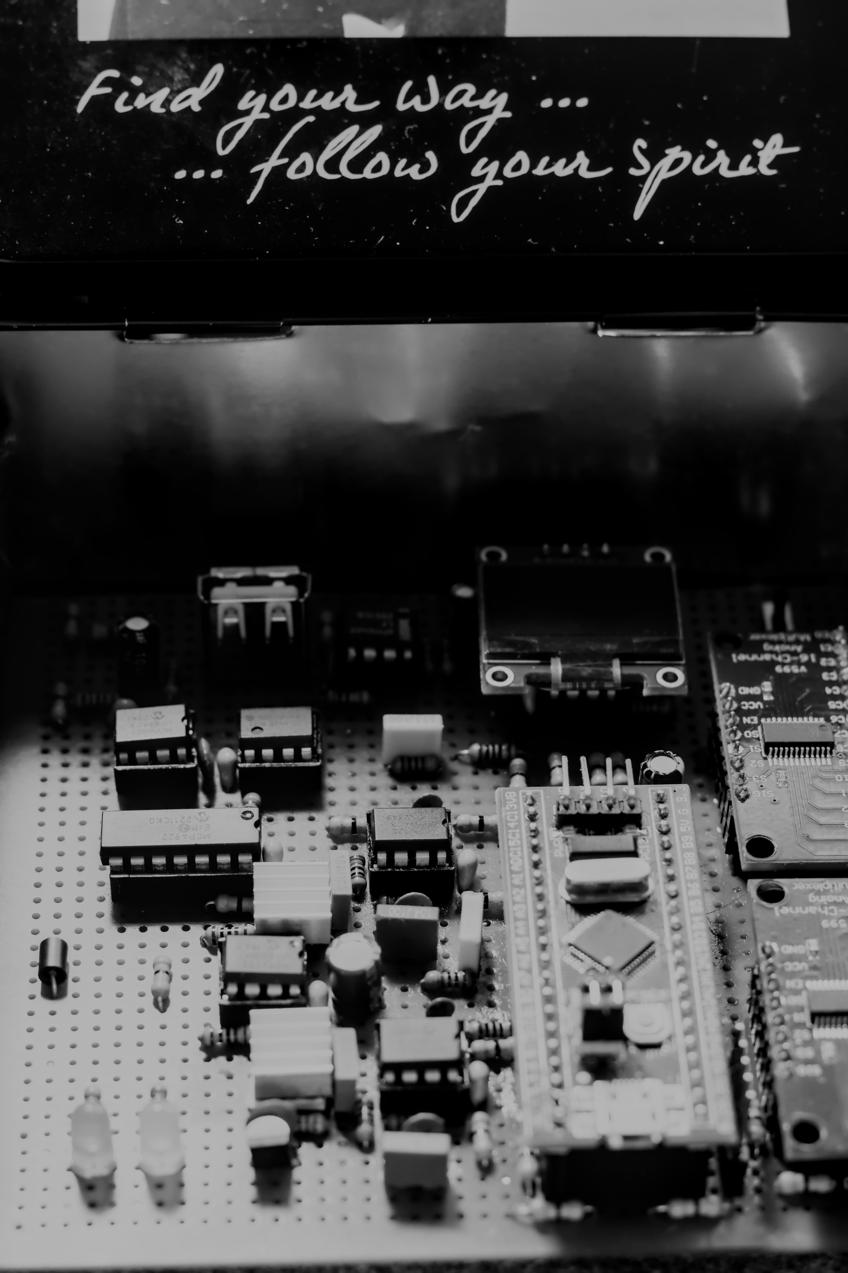
And now I have a circuit that produces 7.8+ bits of entropy, stable after whitening, at military standards. On cheap pertinax, two zener diodes, an STM32 Blue Pill, and a bunch of metal film resistors. It doesn’t look magnificent. But the indeterminacy of the universe works inside it. I can also see the temperature with the DS18.
I call this CTH v.0.1. Can’s Third Hardware. My third hardware.
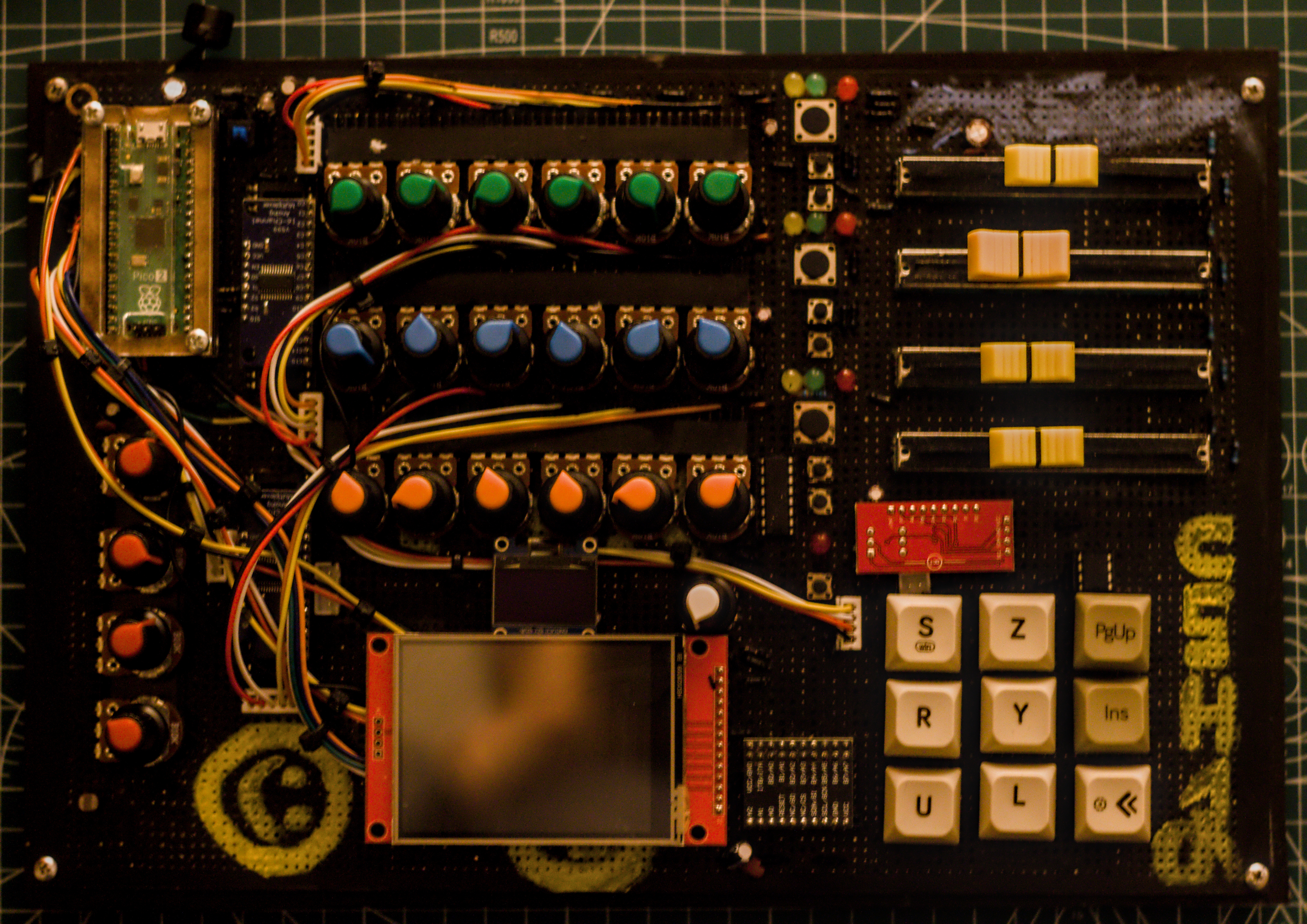
My second hardware, CSH (Can’s Second Hardware), was in a different field — a DAW controller I built for music production. A handmade interface consisting of physical encoders, touchscreen, buttons, and faders, connected via MIDI to Bitwig Studio. A different engineering discipline than CTH, but the same philosophy: Don’t use the ready-made solution on the market, build exactly what you want yourself.
What Will I Do?
Practically, I can use this device for a few things:
For personal purposes.
When I want to generate critical passwords. When a key, a token, needs real entropy — randomness produced not by an algorithm, but by the universe.
When I want to create background noise in Bitwig. A live sound source with a fractal character, different from white noise. Microplasma has its own unique rhythm.
But the real goal, the thing I set in my mind while designing the project: TouchDesigner.
To visualize the indeterminacy of the universe. Let every bit, every sample, turn into a pixel, a movement, a form. Generative visuals fed not by deterministic algorithms, but by real physical events. Let a line appear on the screen the moment the electron tunnels.
It is not certain what life will bring to a person or what it will take away — just as it is not certain what “1” or “0” will come out of this device.
But witnessing something like this in this finite life was a beautiful experience for me. A journey from theory to circuit, extending to the atoms. A process that involved holding a soldering iron in the evenings and falling into a strange silence the moment I said “it works”… plus there was a separate joy in conquering the electrons. 😈😄
It works. And the universe is inside it.
Test
Real Life Demo
Randomness Generation Test
Entropy Quality Test
Code
Update — August 2026
I wrote this post in April 2026 with the first working circuit. Since that day, I have rewritten the firmware from scratch: SP 800-90B continuous health tests, a proper entropy budget, and an AR(16) based analyzer on the host side.
The physics side hasn’t changed — source zeners, mechanism is microplasma + tunneling as I explained in §7. What changed is the proof: the measurement I relied on where I said “I succeeded” (7.9 bits after whitening) shows nothing. The output of a cryptographic hash will be close to 8 bits/byte regardless of the input. The correct measurement should have been done on raw samples before the hash; I did it again, and the number is in the repo.
Firmware (Rust, no_std, embassy)
entirely open:
github.com/caneroglu/cth